Review of Homography

Before reviewing homography, lets first quickly review transformation in 2D and transformation in 3D.

Transformation in 3D

Let us consider a point vector $(x,y)$ in 2D, that is represented by a vector notation $x$. Then we introduce a notation $\bar x$ representing the vector $(x, y, 1)$ which is nothing but the representation of the same $(x, y)$ vector in a slightly different look. The reason for introducing the new notation is to allow single matrix operation to be enough to represent a 3D-transformation, which will be illustrated from the matrix equations below.

The following figure illustrates the basic transformations that occur in 2D plane:

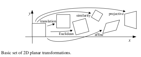
Translation:

2D translations can be written as:

\[\begin{aligned} x' &= \left[ \begin{matrix} I & t \end{matrix}\right] \bar x \end{aligned}\]

Rigid-Body Motion:

2D Rigid body motion or 2D Euclidean transformation (as it preserves Euclidean distances) can be written as:

\[\begin{aligned} x' &= \left[ \begin{matrix} R & t \end{matrix}\right] \bar x \end{aligned}\]

where,

\[R = \left[ \begin{matrix} \cos \theta & -\sin \theta \\ \sin \theta & \cos \theta \end{matrix}\right]\]

Scaled Rotation:

Also known as the similarity transform, this transformation can be expressed as:

\[\begin{aligned} x' &= \left[ \begin{matrix} sR & t \end{matrix}\right] \bar x \end{aligned}\]

Or,

\[\begin{aligned} x' &= \left[ \begin{matrix} a & -b & t_x \\ b & a & t_y \end{matrix}\right] \bar x \end{aligned}\]

Affine Transformation:

The affine transformation is written as $x’ = A\bar x$, where $A$ is an arbitrary $2 \times 3$ matrix, i.e.

\[\begin{aligned} x' &= \left[ \begin{matrix} a_{00} & a_{01} & a_{02} \\ a_{10} & a_{11} & a_{12} \end{matrix}\right] \bar x \end{aligned}\]

Projective Transformation (Homography):

This transformation operates on homogenous coordinates (represented here as tilde over the variable as in $\tilde x$),

\[\begin{aligned} \tilde x' &= \tilde H \tilde x \end{aligned}\]

where, $\tilde H$ is an arbitrary $3 \times 3$ matrix. Also note that $\tilde H$ is homogenous and hence two $\tilde H$ matrices that differ only by scale are equivalent.

Transformation in 3D

Similarly, the transformations in 3d is summarized in the image below:

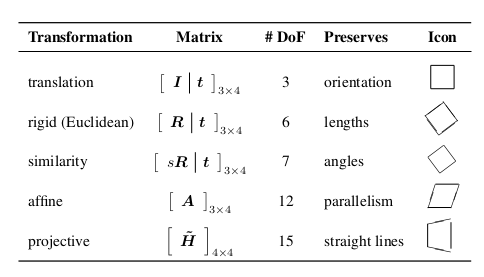
Note that the notations with the bar sign represent operations on normal coordinates and that with the tilde sign represent homogenous coordinates.

3D-to-2D Projective Transformation:

In applying projective to the imaging process, it is customary to model the world as a 3D projective space $\mathbb R^3$ and similarly, the model for the image is the 2D projective plane $\mathbb R^2$. Central projection is simply a map from $\mathbb R^3$ to $\mathbb R^2$. If we consider points in $\mathbb R^3$ written in terms of homogenous coordinates $(X, Y, Z, T)^T$ and let the centre of projection be the origin $(0, 0, 0, 1)^T$, then we see that the set of all points $(X, Y, Z, T)^T$ for fixed $X$, $Y$, $Z$, but varying $T$ is irrelevant to where the point is imaged. In fact, the image point is the point in $\mathbb R^2$ with homogenous coordinates $(X, Y, Z)^T$.

Thus the mapping may be presented by a mapping of 3D homogenous coordinates, represented by a $3 \times 4$ matrix $P$ with the block structure $P = \left[ \begin{matrix}I_{3 \times 3} \vert O_3 \end{matrix}\right]$

When the centre of projection and projection plane are arbitrary, the most general projection is given by:

\[\begin{aligned} \left(\begin{matrix} x \\ y \\ w \end{matrix}\right) = P_{3 \times 4} \left( \begin{matrix} X \\ Y \\ Z \\ T \end{matrix}\right) \end{aligned}\]

Furthermore, if all the points lie on a plane (we may choose this as the plane $Z=0$), then the linear mapping reduces to

\[\begin{aligned} \left(\begin{matrix} x \\ y \\ w \end{matrix}\right) = H_{3 \times 3} \left( \begin{matrix} X \\ Y \\ T \end{matrix}\right) \end{aligned}\]

which is a projective transformation. Following image illustrates the concept.

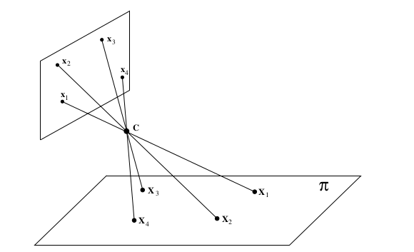
Here all the space points are coplanar, hence there is a projective transformation between world and image planes. (i.e. $x_i = H_{3\times 3} X_i$)

Multi-View Reconstruction

Suppose we have more than one (say two for now) camera matrices, $P$ and $P’$. Let $x_i’\leftrightarrow x_i’$ be correspondences in two images. If $X_i$ is the set of 3D points, then we have $P X_i = x_i$ and $P’ X_i = x_i’$.

However neither the camera matrices (i.e. the projection matrices $P$ and $P’$) are known and nor are the point $X_i$, and that’s what we are here for.

No matter how many image we are given, it is impossible to tell the absolute position of the objects in the image and are best expressed at best up to as similarity transformation of the world (Refer paragraph above for similarity transformation). However, it turns out that unless something is known about the calibration of the two cameras, the ambiguity in the reconstruction is expressed by a more general class of transformations - projective transformations.

Mathematically, the ambiguity arises because the equation $P X_i = x_i$ can be expressed for a camera $j$ as:

\[\begin{aligned} P_jX_i = \left(P_jH^{-1})(H X_i\right) \end{aligned}\]

The $4\times 4$ matrix $H$ represents an arbitrary projective transformation and we say that the reconstruction has a projective ambiguity or is a projective reconstruction.

References:

• Multiple View Geometry in Computer Vision (R. Hartley, A. Zisserman)
• Computer Vision : Algorithm and Application (R. Szeliski)

PS:

Parts of the article is inspired from the references and is presented as is and with some modification. No infringement of copyright is intended.

---

Last Updated: Sunday, 6th September, 2020, 16:21:52 NPT Author: Madhav Humagain (scimad)