Summary of ResNet Paper
Resnet
The ResNet Paper (Deep Residual Learning for Image Recognition (Microsoft Research)) Summary:
Introduction:
- Deep networks naturally integrate multilevel features and classifiers in an end-to-end multilayer fashion, and the “levels” of features can be enriched by the number of stacked layers (depth).
- Network depth is of crucial importance.
- Very deep networks have the problem of vanishing/exploding gradients but this has been largely addressed by normalized initialization and intermediate normalization layers.
- A problem called “degradation” occurs in deeper networks which is different from error due to over-fitting and adding more layers doesn’t help.
- Though an more optimal solution to learning problems exist, current (prior?? with reference to the paper) aren’t able to find such solutions.
- ResNet paper addresses the degradation problem by introducing a “deep residual learning” framework.
Instead of letting the stacked layers directly fit a desired underlying mapping, the layers are let to fit a residual mapping.
Desired underlying mapping \(H(x)\), we let the stacked nonlinear layers fit another mapping of \(F(x):= H(x)-x\). The original mapping is recast into \(F(x)+x\).
- The hypothesis is that, it is easier to optimize the residual mapping than to optimize original, unreferenced mapping.
- \(F(x)+x\) can be realized in network by feed-forward networks with shortcut connections (identity mapping) and adding to outputs of stacked layers. It doesn’t add computational complexity, nor parameters of network.
- Trained using end-to-end SGD with backprop.
- Easy to optimize without introducing degradation issue unlike other (plain) networks.
- Accuracy gains from increased depth, producing better results on Imagenet (and similar on CIFAR-10).
- Models trained over 100 layers and experimented over 1000 layers.
- 152 layer residual network (resnet) is (at the time of this paper) the deepest network ever presented on Imagenet and has 3.57% top-5 error.
- Excellent generalization performance.
Deep Residual Learning and Short Connections:
Residual Representations
- Vector of Locally Aggregated Descriptors (VLAD) and Fischer Vector (probabilistic representation of VLAD) encodes residual vectors and are powerful shallow representation for image retrieval and classification.
- Encoding residual vectors are effective than encoding original vectors.
- Solvers that rely on residual vectors converge much faster than standard solvers that are unaware of the residual nature of solutions which suggests that good reformulation or preconditioning can simplify the optimization.
Shortcut connections
- Connections from intermediate layers are directly connected to auxiliary classifiers for addressing vanishing/exploding gradients.
- The “inception” paper showed the use of shortcut branches and a few deeper branches to create an “inception” layer.
- “Highway networks” present shortcut connections but those have parameters whereas resnet’s shortcuts are parameter-free. Also, When “closed” (approaching zero) the shortcut, the layers in highway networks represented non-residual functions, whereas resnet shortcuts (identity) are never closed, and all information is always passed through, with additional residual functions being learned.
- Resnet have accuracy gains unlike in highway networks upon increasing depths.
Residual Learning
- Consider \(H(x)\) as an underlying mapping to be fit.
- If non linear layers can approximate \(H(x)\), it could also do same for \(H(x)-x\)
- Rather than expect stacked layers to approximate H(x), we explicitly let these layers approximate a residual function \(F(x) := H(x) − x\). Though both forms can be approximated by non linear layers, the ease of learning might be different.
-
While adding layers, in doing so, the error must not exceed the shallower counterpart because if the added layer could learn identity mapping, there should be no net effect of adding the layer in the actual learning of model. The existence of “degradation problem” suggests that solvers have difficulty in approximating the non-linear layers to identity mapping.
- In residual mapping, if the optimal mapping is identity, then the weights are driven towards zero, so that the output (with shortcut connection) simply approaches to identity mapping. In reality, such identity mappings are not optimal and there is space for the network to learn. What residual network thus gives is a precondition (or initial state with all weights zero.(?)) to learn more optimal function. This comes from the mathematical statement: “If the optimal function is closer to an identity mapping than to a zero mapping, it should be easier for the solver to find perturbations with reference to an identity mapping, than to learn the function as a new one.”
- Experiments show that such identity mapping provide reasonable preconditioning.
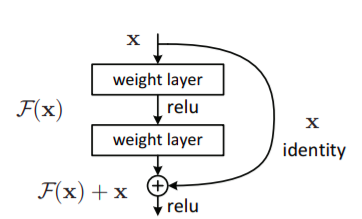
Mathematics for shortcuts
- Residual learning is applied to every few stacked layers (as shown in the above figure) (applies also for conv. layers, not just fully-conn. layers).
- A building block defined mathematically as: \(y=F(x, {W_i})+x\) where \(F(x, {W_i})\) represent the residual mapping (or let’s say zero mapping, so that the whole block gives approximately an identity mapping, or we can take identity mapping as reference) to be learned.
- \(F+x\) is element-wise addition and non linearity is applied afterwards as shown in figure above. The dimensions of \(x\) and \(F\) must be equal and can be made so using “linear projection” or using appropriate matrix multiplication by \(W_s\) [i.e.\(y=F(x,{W_i})+W_sx\)] in otherwise case.
Network Architectures
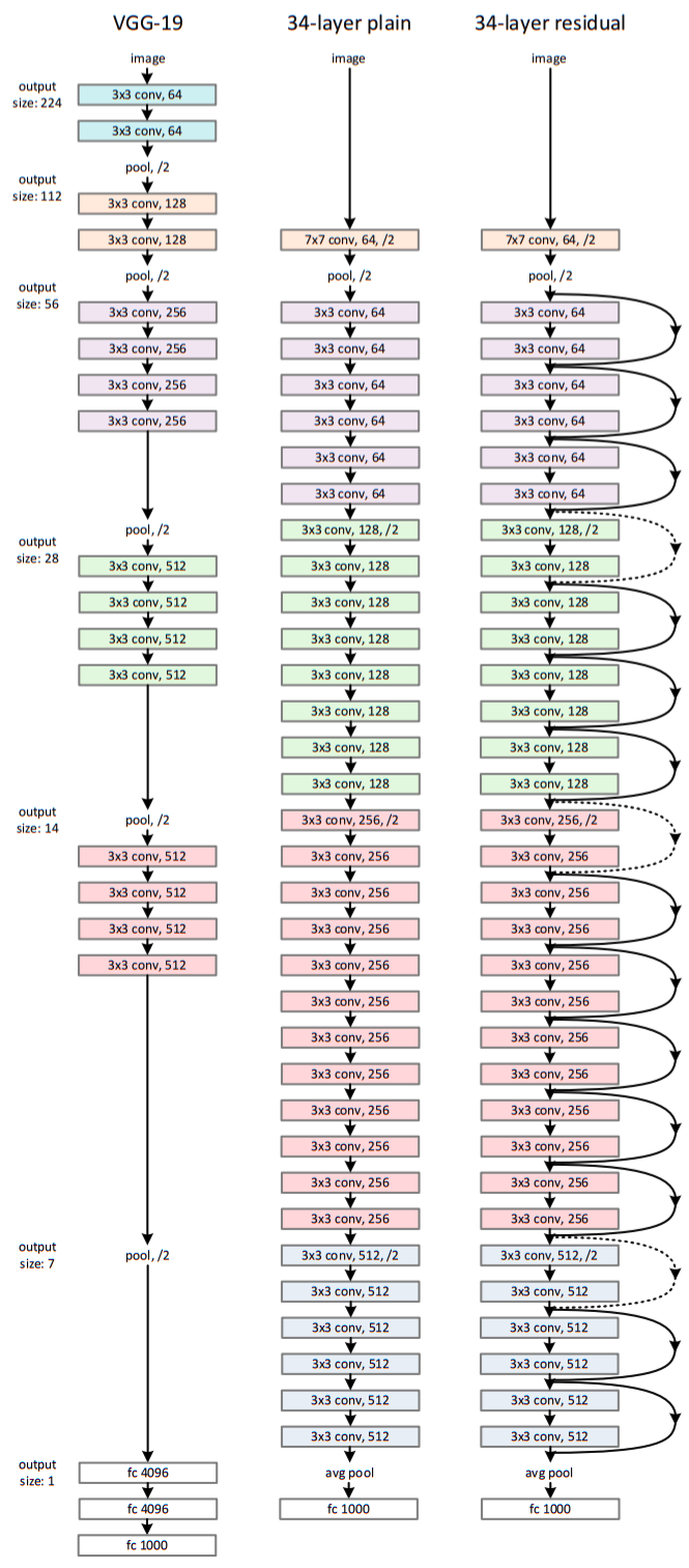
- The (plain) baseline models are inspired by VGG nets.
- The conv. layers have 3x3 filters.
- For the same output feature map size, the layers have the same numbers of filters. If the feature map size is halved, the number filters is doubled. This preserves the time complexity per layer.
- Down-sampling directly by conv. layers with stride of 2.
- Global average pooling layer and 1000-way FC layer with softmax at the end of layer.
- Total 34 weighted layers ( as shown in middle of the above figure).
- Lower complexity and only 18% FLOPS than VGG-19.
- Based on the plain network, connections are inserted. (connection of same dimension shown in solid and otherwise in dotted arrows.) While dimensions are added, either extra zero are padded of matrix method is used to increase dimension as said earlier.
Their Implementation
For imagenet:
- resized with its shorter side sampled in [256,480] for scale augmentation.
- 224x224 crop is sampled from image or it’s hor. flip
- per-pixel mean subtracted.
- Standard color augmentation used.
- Batch normalization right after each conv. and before activation.
- Trained from scratch, using SGD with mini-batch of 256
- Learning rate from starting 0.1, divided by 10 as error tends saturation
- 600000 iterations, weight decay of 0.0001, momentum of 0.9 and dropout not used.
- Testing done by averaging the scores in different scales such that shorter side is in {224, 256, 384, 480, 640}.
ImageNet Detection (DET)
- Pretrained on 1000-class ImageNet classification set and fine-tuned on DET data.
ImageNet Localization (LOC)
- Classify and localize objects
- First image-level classifiers are adopted
- Localization algorithm only accounts for predicting bounding boxes based on predicted classes.
- Per-Class-Regression for learning bounding box for each class.
- Pre-train the networks for ImageNet classification and then fine-tune them for localization.
- Train networks on the provided 1000-class ImageNet training set.
- Localization is based on Region-Proposal-Network (RPN) with few modifications.
- RPN ends with two sibling 1x1 conv. layers for binary classification (cls) and box regression (reg) both designed in per-class form.
- Binary classification layer has a 1000-d output and each dimension is a binary logistic regression for predicting being or not being an object class.
- The Box-Regression (reg) layer has a 1000x4-d output consisting of box regressor for 10000 classes.
- Random sampling of 224x224 crops for data augmentation.
- Mini-batch size of 256 for fine tuning.
Last Updated: Monday, 23rd November, 2020, 09:34:29 NPT Author: Madhav Om (scimad)